Internal and external balance under floating excha...
According to our analysis of the Swan diagram, by combining an exchange rate change with expenditure changing policy it is possible to achieve both internal and external balance.An interesting issue that we can explore within the framework of our model is what are the likely differences of achieving internal and external balance by combining exchange-rate changes with monetary policy, as opposed to combining them with fiscal policy.Figure 3.5 illustrates the case of monetary expansion under floating exchange rates.Initial equilibrium is at point A with interest rate r1 and output level Y1.The authorities adopt an expansionary monetary policy and this shifts the LM schedule from LM1 to LM2.The combination of a fall in the interest rate and increase in income leads to a balance-of-payments deficit at point B.However, the exchange rate is allowed to depreciate and this leads to a rightward shift of the IS schedule from IS1 to IS2 and a rightward shift of the BP schedule from BP1 to BP2.However, it also leads to a leftward shift of the LM schedule until all three schedules intersect at a common point such as C with new income level Y2 and interest rate r2.Hence, by using monetary policy in conjunction with exchange-rate changes, it is possible to raise real output to the full employment level and achieve external balance simultaneously.
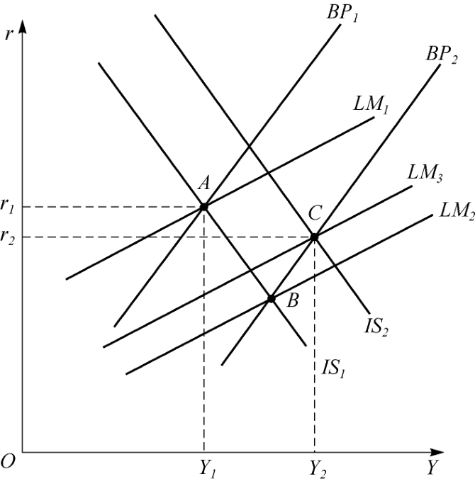
Figure 3.5 A monetary expansion under floating exchange rates
Overall, the money supply expansion results in an exchange-rate depreciation, a fall in the domestic interest rate, and an increase in income.The lower interest rate implies a lower capital inflow/higher capital outflow than before the money supply expansion, while the increase in income worsens due to the exchange rate depreciation.It must have improved because the capital account has deteriorated due to the fall in the domestic interest rate.
Fiscal expansion under floating exchange rates
The effects of a fiscal expansion on the exchange rate under floating rates depend crucially upon the slope of the BP schedule relative to the LM schedule.We shall consider two cases: In case 1 the BP schedule is steeper than the LM schedule, while in case 2 the reverse is true.
In Figure 3.6 the BP schedule is steeper than the LM schedule, which means that capital flows are relatively insensitive to interest-rate changes, while money demand is fairly elastic with respect to the interest rate.An expansionary fiscal policy shifts the IS schedule from IS1 to IS2.The induced rise of the domestic interest rate and domestic income has opposing effects on the balance of payments; the expansion in real output leads to a deterioration of the current account, but the rise in interest rate improves the capital account.However, because capital flows are relatively immobile moves into deficit.In turn, the deficit leads to a depreciation of the exchange rate and this has the effect of shifting the BP schedule to the right from BP1 to BP2 and the LM schedule to the left from LM1 to LM2 and the IS schedule even further to the right from IS2 to IS3.Final equilibrium is obtained at point C, with interest rate r2 and income level Y2.Hence, the deterioration in the balance of payments resulting from the rise in real income is offset by a combination of a higher interest rate and an exchange-rate depreciation.
In Figure 3.7 an expansionary fiscal policy shifts the IS schedule from IS1 to IS2.In this case because capital flows are much more responsive to changes in interest rates the BP schedule is less steep than the LM schedule.The increased capital inflow more than offsets the deterioration in the current account due to the increase in income, and the balance of payments moves into surplus.The surplus induces an appreciation of the exchange rate which moves the LM schedule to the right from LM1 to LM2, the BP schedule to the left from BP1 to BP2, and the IS schedule to the left from IS2 to IS3.Equilibrium is obtained at a higher level of output, higher interest rate and an exchange-rate appreciation.
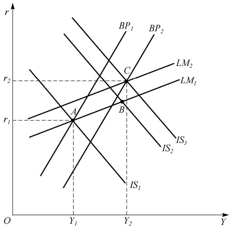
Figure 3.6 Case 1: fiscal expansion under floating exchange rates
Hence a fiscal expansion can, according to the degree of international capital mobility, lead to either the exchange-rate depreciation or an exchange-rate appreciation.
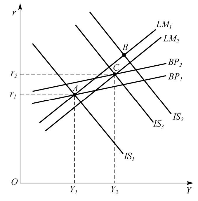
Figure 3.7 Case 2: fiscal expansion under floating exchange rates