4.2 The Smart Growth Plan Over Next Few Decades
4.2.1 The Development Roadmaps of The Smart Growth of Two Cities
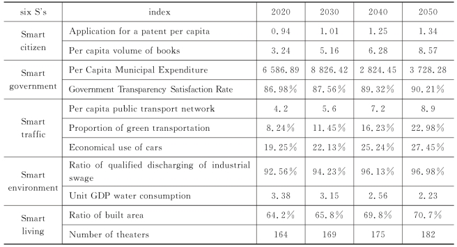
Thinking of the weakness of the growth plans of the two cities,we develop a new growth plan for both cities over the next few decades.Taking the geography,expected growth and economic opportunities into consideration,the connective index of the six S's metric system is given in the Table 15 and Table 16.
Because the data is too big,so we take several indexes from every standards as an example.
Table 15 The new growth plan of Arlington
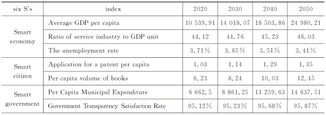
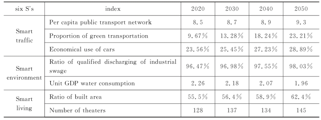
On the basis of the index value we have set up,the redesigned growth plan can be displayed by the style of roadmap.And the redesigned smart growth plan is shown in the Figure 7 and Figure 8.
It is vividly shown in the roadmap that Sanya should focus more on the economic development in next 10 to 20 years.The society development and the environment development are mainly enhanced in later years.
The economic development in Arlington tends to be a steady growth,not as fast as the Sanya's.One of the most important part of the total growth plan is the environmental development.It is vividly shown in the picture that some part of the environmental plan covers almost the whole period of time.
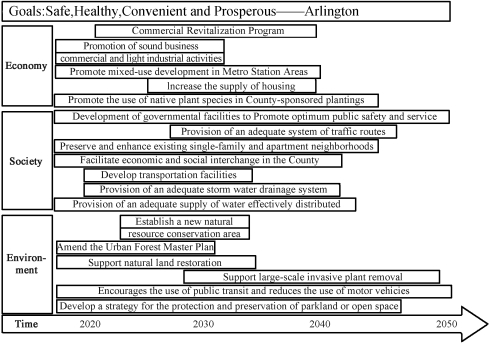
Figure 7 The development roadmap of Arlington in decades
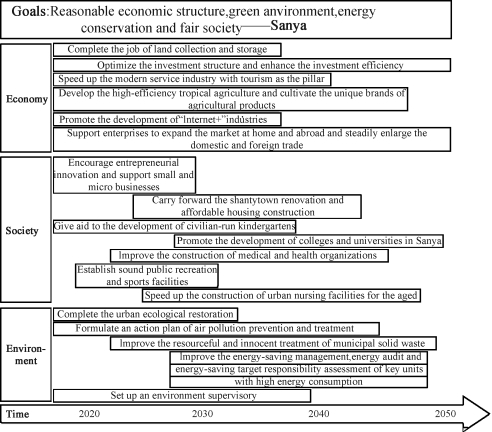
Figure 8 The development roadmap of Sanya in decades
4.2.2 Evaluation of The Redesigned Growth Plan
Now that,we have build up the roadmap of the two cities to show the further growth of the cities.It is also necessary to evaluate the redesigned growth plan to clarify whether it is feasible and the potential of individual initiatives.
In this part,we plan to build up a growth model to simulate the real situation.Then we should evaluate the redesigned growth plan as the program above.Finally,we compare the evaluated values with the simulated values,and the potential of individual initiatives can be represent by the difference between the two values.And the main method of evaluation is clearly displayed in the Figure 9.
Table 16 The new growth plan of Sanya

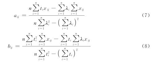
To build up the growth model,firstly we assume that the variation function with the time is presented as follows:
![]()
Where,1<x<6,1<j<50,and aij,bij is the constant value calculated by the least square method.
Assuming that we take the smart economy as an example.After the variation function of the second-grade index with the time is set up,the relation function between the smart economy and the second-grade index is presented as follows:
![]() (https://www.daowen.com)
(https://www.daowen.com)
Where,ci represents the weight of the second-grade index,c 0 represents the constant value.
The theoretical values of smart economy from 2000 to 2006 are calculated according to Function(1)and(2)and then compared with the practical values as shown in the following table.
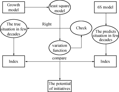
Figure 9 The progress of the evaluation of the developed growth plan
According to the sheet above,we can analyze the error of the equation.From the table above,it can be seen that there exists a certain difference value between the theoretical values and the practical values,so the error analysis is quite necessary.Given that the error of the growth model isβ,its value is:

Table 17 The theoretical and practical value of smart economy
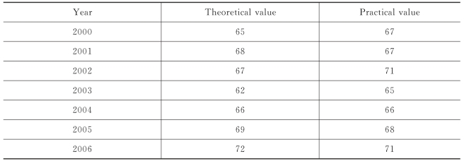
After calculating,theβis 4.23%.If the error is less than 5.00%and the growth model is in accordance with the practical growth,the model can be used to determine the development trend of the practical values in the future.
To sum up,the growing trend of six first-grade indexes with the time is shown in the following table.
And according to the roadmap model above,we can get the evaluation value of the resigned growth plan,which is shown in the following Table 18.
Table 18 The true value predicted by the growth model
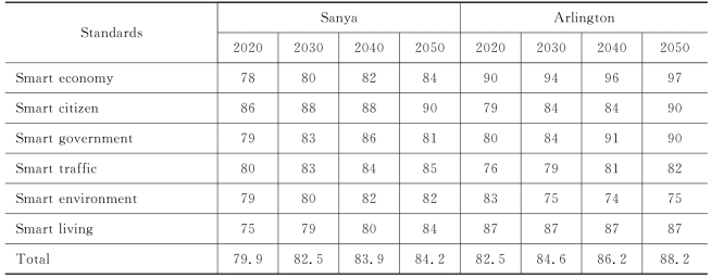
Table 19 The smart index of new growth plan over next several decades
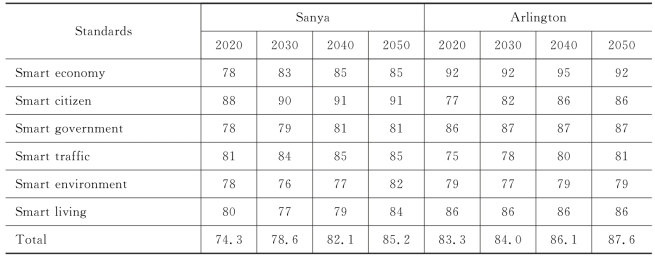
Assuming the value of growth model sti is the true situation,and the value of the evaluation sei is the situation after conducting the redesigned growth plan.So the potential p i can be represented as the following equation:
![]()
So,after combining the Table 17 and the Table 18,we can get the potential value of all the indexed in different years.
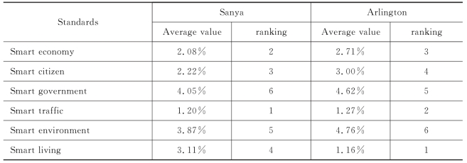
According to the table above,we can calculate the time averaged deviation.And then,we use the average deviation to represent the potential of the individual initiatives.And the higher the deviation is the lower the potential.The final ranking can be seen in the Table followed.
It is clearly shown in the table that the smart traffic is the most possible to be realized to Sanya and the smart living is the most possible to be realized to Arlington.And the potential between the two cities can be seen as similar.
Table 20 The deviation of individual initiatives
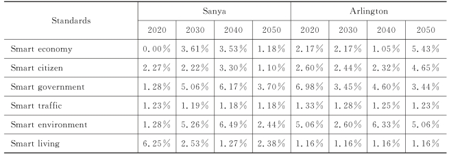
Table 21 The ranking of individual initiatives
